
Microsphere projection
Microsphere projection is an method of interpolating Cartesian data based on the physical model of an infinitely small sphere located at the point of interpolation. This tiny sphere is then ‘illuminated’ by the surrounding sample points. Based on the degree of illumination on various parts of the sphere by various sample points, a series of weights for all the sample points are assigned. These weights, when applied, yield an interpolated value for the location.
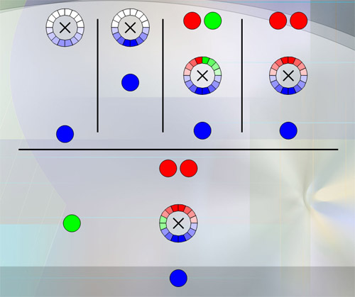
Algorithm implementation
Defining the sphere
The surface of the microsphere is divided into a large number of equally-spaced regions. Each region records for itself which sample point has illuminated it the most, and what illumination that sample point has provided. Each surface region is represented by a single unit vector pointing out from the center of the sphere to the center of that region. “S[i].Vector” will be used to represent the unit vector for surface region i. The more regions used, the greater the precision of the interpolation.
For each region, two values are recorded: one recording the index of which sample point has illuminated this section the greatest, and the second recording the degree of illumination from this point. These will be referred to as “S[i].Brightest_Sample” and “S[i]. Max_Illumination”, respectively.
Since determining an arbitrarily large number of equally-spaced regions on the surface of a sphere is no small task, we accept that a large number of randomly placed unit vectors will provide a fairly uniform distribution.
The vectors are generated using the following algorithm:
do
// x,y,z are uniformly-distributed random numbers in the range (-1,1)
x := rand(-1,1)
y := rand(-1,1)
z := rand(-1,1)
vectorSize := sqrt (x*x + y*y + z*z)
// if the vector these points form is outside the unit sphere,
// disregard and find a new vector.
while ( vectorSize > 1 )
// normalize the vector, so that it forms a unit vector for the surface of our sphere.
x := x / vectorSize
y := y / vectorSize
z := z / vectorSize
Sample point projection
Net illumination is applied to the microsphere by iterating through each of the sample points, and applying illumination to the sphere one-by-one. It should be noted that illumination on various parts of the sphere decreases proportionally to the acuteness of the angle between the surface of the sphere and the direction of the sample point. Illumination also decreases as the distance between the microsphere and the sample point increase. Much like Shepard’s Method, this inverse relationship between distance and ‘brightness’ is governed by a power value ‘p’ specified by the user where p>0, p=1 and p=2 are typical values. p=1 yields an interpolation that is C0 (non-differentiable), p > 1 is C1 (first-derivative is continuous). Similar to Shepard’s Method, when p>>2, the closest points dominate the interpolation and the algorithm becomes the equivalent of Nearest Neighbor.
Intesnsity projection function:
for i := 0 to Number of Samples
// vector connecting the current sample to the interpolation location
vector1 := sample[i].XYZLocation - interpolation.XYZLocation
// the distance-modified weight of this point
// p > 0, typically p=1 or p=2.
weight := pow(vector1.Size, -p)
// the value of ‘Precision’ represents how many subdivisions
// of the surface of the microsphere we are working with.
for j := 0 to Precision
// each sample only 'shines' on one hemisphere.
// as the angle becomes more acute, the intensity
// of that shine decreases as the cosine function
cosValue := CosValueBetweenVectors(vector1, S[j].Vector)
// if the brightness of the shine on this section of the sphere
// is more than any other point thus far checked, update our
// 'Brightest_Sample' and 'Illumination' data.
if (cosValue * weight > S[j].Max_Illumination)
S[j].Max_Illumination := cosValue * weight
S[j].Brightest_Sample := i
endif
endfor
endfor
Accumulation of the final values from the sphere
Once all the calculations are complete regarding the maximum illuminations on the various sections of the sphere, we must make use of this data to produce a single interpolated value. To do this, we assign a weight to each sample point equal to the total illumination that point provided to the sections of the sphere. Note that each section of the sphere only records data regarding the point which provided the most illumination; sample points which did not out-shine any other points on any section of the sphere are assigned a weight of 0.
Accumulation pseudo-code:
// accumulate the data from our sphere, and determine final interpolation
value := 0
totalWeight := 0
for i := 0 to Precision
value := value + S[j].Max_Illumination * sample[S[j].Brightest_Sample].SampledValue
totalWeight := totalWeight + S[j].Max_Illumination
endfor
// the final interpolated value generated by the algorithm
interpolation := value / totalWeight
Mathematical form
w_i=\max\left\{\left\|\ell_j-I\right\|^{-p}\cos\left(s_i,\ell_j-I\right):j\in\left\{1,2,3,\dots,N\right\}\right\}
m_i=\mbox{any }v_j:\left[\left(\left\|\ell_j-I\right\|^{-p}\cos\left(s_i,\ell_j-I\right)=w_i\right)\land j\in\left\{1,2,3,\dots,N\right\}\right]
f(I)=\begin{cases}
v_i\mbox{ if }\exists{i}\in\left\{1,2,3,\dots,N\right\}\left(I=\ell_i\right)\\
\displaystyle\frac{\displaystyle\sum_{i=1}^{P}m_iw_i}{\displaystyle\sum_{i=1}^{P}w_i}\mbox{ otherwise }
\end{cases}
I = \mbox{Location of interpolation}
p = \mbox{Propagation of influence power, } p>0
v_i = \mbox{Value of sample }i,~i\in\left\{1,2,3,\dots,N\right\}
\ell_i = \mbox{Location of sample }i,~i\in\left\{1,2,3,\dots,N\right\}
N = \mbox{Number of samples}
s_i = \mbox{Evenly spaced unit vector on surface of sphere,}~i\in\left\{1,2,3,\dots,P\right\}
P = \mbox{Precision (number of unit vectors on sphere),}~P\gg2d
d = \mbox{Dimensionality of data (}d=2\mbox{ is planar)}
Useful properties of microsphere projection
Multi-dimensional
MS Projection works in any Cartesian coordinate system. The algorithm works as well in 1 dimension as it does in 10 or 20 dimensions.
Maximum principle
MS Projection exhibits the maximum principle. In other words, the interpolated value is guaranteed to lie in the range between the minimum sampled value and the maximum sampled value. Other interpolation techniques which demonstrate this quality include Nearest Neighbor interpolation, and Shepard’s Method (naïve inverse-distance weighting). This feature was chosen because it is guaranteed to provide intuitive results for bounded data.
Preservation of monotonic behavior
MS Projection is guaranteed to preserve monotonic and strict monotonic behavior over any set or subset of sample points. For example, if the set or subset of sample points is increasing or strictly increasing over a range, then the interpolation is guaranteed to be increasing or strictly increasing over the same range.
No oscillatory behavior
MS Projection demonstrates no oscillatory behavior between sample points, unlike functional approximations which are designed to preserve high differentiability.
Stable extrapolation ability
MS Projection provides a stable extrapolation ability. Functional approximations tend to produce extremely volatile extrapolation results beyond the range of the data points. This can cause serious issues in higher dimensions where the differentiation between interpolation and extrapolation within the volume is difficult to determine. Because MS Projection provides a stable extrapolation, it has considerable benefits over functional approximations when visualizing higher dimensional data.
Drawbacks of microsphere projection
Differentiability class
MS projection is class C1 only ifp > 1, and C0 otherwise. This means that the interpolation will have a continuous first derivative, however no guarantees are made of the second derivative of the interpolation. MS Projection may actually be better than C1, but furhter research must be done.
Maximum principle
Depending on the nature of the problem, the fact that MS projection exhibits the maximum principle can be an issue. That the interpolation method is unable to interpolate a value beyond the minimum and maximum sampled values can cause problems depending on the context.
Run time
Depending on the size of the data set and other considerations, MS projection can require more computation time than some of the other interpolation algorithms. Though the overall runtime is O(PN), this set of calculations must be run every time a point is to be interpolated. Radial Basis Function (RBF) interpolations such as thin plate spline, multiquadric, and volume spline are all O(N 2) for the first interpolation and O(N) (with a very small overhead) for subsequent interpolations.
First-derivative behavior near sample points
As interpolation location approaches a sample point, the first derivative in all dimensions approaches 0 when p>1. In most contexts this is undesirable behavior; however it is necessary if we wish to preserve the Maximum Principle in conjunction with differentiability.
References
- Dudziak, William J., "Presentation and Analysis of a Multi-Dimensional Interpolation Function for Non-Uniform Data: Microsphere Projection", Master’s thesis, Akron, Ohio, 2007.
- Freedman, S. and Adams, J., "HUMAN-INSPIRED ROBOTIC FORGETTING: FILTERING TO IMPROVE ESTIMATION ACCURACY", IASTED: Robotics and Applications, 2009.
See also
- Interpolation
- Thin plate spline
- Spline interpolation
External links
- Step-By-Step Algorithm Walkthrough
- Apache Foundation JAVA implementation of Microsphere Interpolation
- Powerpoint Presentation Regarding Microsphere Projection
- Microsphere Projection Tutorial